Tharp's Thoughts Weekly Newsletter (View On-Line)
-
Article Why Band Trading Works, Part 2 by Ali Moin-Afshari
-
-
Trading Tip A Deeper Look at Unemployment Numbers: Part 2 by D.R. Barton, Jr.
-
Gold Report Gold Analysis and Strategy by Florian Grummes
Ken Long Teaches 3 Systems Workshops this Summer
In July, you will have the opportunity to learn longer-term trading systems at Ken's Core Trading Systems Workshop. Then, the next month, you can attend the new Day Trading Systems Workshop, along with it's hands-on counterpart, Live Day Trading.
Don't miss out, these workshops tend to sell out. If you wish to attend, register now to reserve your seat.
Click here for more information about these and other workshops.
 Why Band Trading Works Why Band Trading Works
Part 2 - Bands
by Ali Moin-Afshari
View On-line
In part 1, we laid down the foundation for band trading by reviewing the concept of trends and trend analysis. In this article, we will study some popular bands and channels. We’ll also analyze how bands can improve the reliability of signals without altering the overall trend profile and how they could be used to slow down trading without sacrificing the biggest profits. The time of greatest indecision is the point of trend change, when traders get whipsawed the most. A simple way to avoid frequent false signals is by using a band.
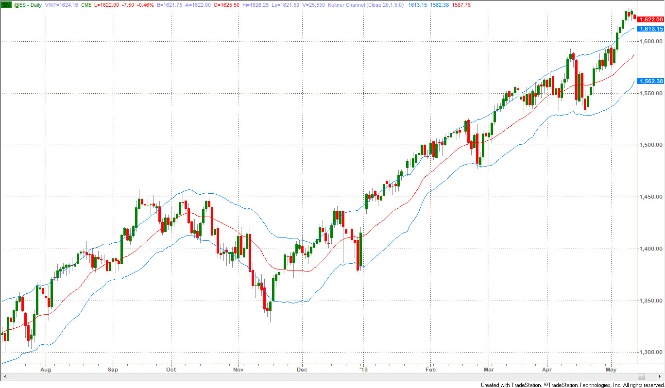
Keltner Channel
The original Keltner Channel was named after a Chicago-based corn trader, Chester W. Keltner. Keltner used a ten-day simple moving average of typical price, TP=(High+Low+Close)/3, as the center line and built a band around it by plotting a line above it using the simple moving average (SMA) of highs and a line below using SMA of lows. All three simple moving averages used the same look-back period of 10 days. That original version of the Keltner Channel is no longer in use. The modern Keltner Channel uses either SMA or EMA (Exponential Moving Average) for the center line and Wilder’s ATR (Average True Range) multiplied by a volatility factor to create the bands.
Fig.1 shows Keltner Channel applied to the chart of S&P500 e-mini futures.
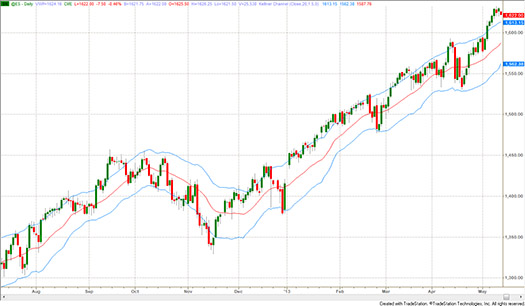
Figure – 1: Keltner Channel plotted on a 9-Month Daily Chart of ES:
20-period Moving Average, F=1.5 ATR
(click here to see a high-resolution version of this chart)
The Keltner channel is used in two ways:
- to identify breakouts for trend following, and
- to find overbought/oversold price levels within trading ranges.
Bollinger Bands: a Variety of Volatility Bands
The problem with using ATR is its slow response to changes in volatility. Creating a band that is responsive to volatility can improve the reliability of trend signals. There are many methods from which to choose, though all of these methods use a constant value as a multiplier or scaling factor for scaling.
The volatility multiplier or factor increases or reduces the sensitivity of the band to changes in price. In simple mathematics, if “s” is a scaling factor and “p” is a fixed percentage, then the following bands can be constructed:
| Percentage of Trendline |
Band = MA ± s x p x MA |
| Percentage of Price |
Band = MA ± s x p x Price |
| Average True Range |
Band = MA ± s x ATR of previous bar x MA |
| Standard Deviation |
Band = MA ± s x STDev of previous bar x MA |
In the above formulas, MA is the moving average of price and Band is the value calculated for plotting the band on the price chart. To calculate both bands (up and down from the MA), two values must be calculated using +s and –s, therefore ±s.
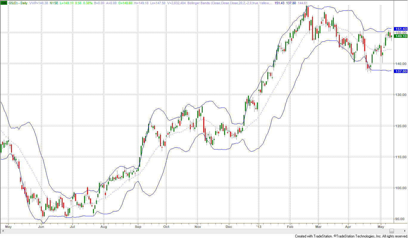
A robust measurement of price volatility is the standard deviation of the price itself, calculated over a period of recent price history, which is the last formula listed above. John Bollinger popularized the combination of a 20-day simple moving average with bands formed using 2 standard deviations of price changes over the same 20-day period and they are now frequently called Bollinger Bands.
Because the standard deviation represents a confidence level and prices are not normally distributed (i.e. due to fat tails in price action of financial markets), the choice of two standard deviations produces an 87% confidence band. If prices were normally distributed, two standard deviations would have equated to 95.4% of the price action range. Trading systems based on Bollinger Bands are usually combined with other techniques to identify extreme price levels.
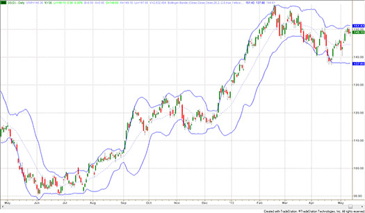
Figure – 2: Standard Bollinger Bands on a One-Year Daily Chart of GS
Simple Moving Average 20, ±2 Standard Deviations
(click here to see a high-resolution version of this chart)
Characteristically, once trending prices move outside either the upper or lower Bollinger Band, they can remain outside for a number of days in a row. This type of behavior is called “crawling up the bands” and is typical of what is also called “high momentum.”
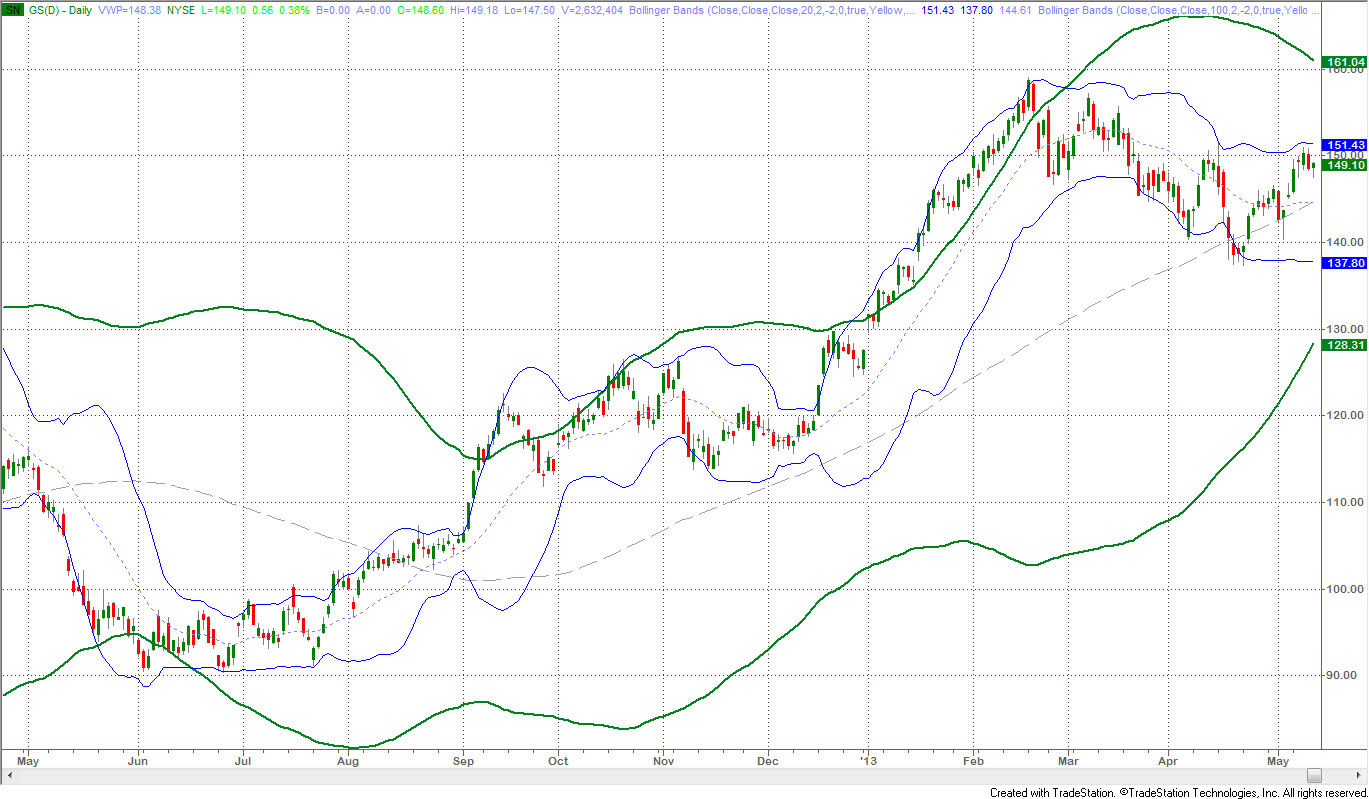
Note that the width of the band varies considerably with the volatility of prices and that a period of high volatility causes a “bubble”, which extends past the period where volatility declines. Bollinger Bands are excellent for showing the cyclical nature of volatility: low volatility begets high volatility and vice-versa. It is also possible to apply Bollinger Bands to different time frames to clarify major and minor trends in the market as shown in the chart below which combines weekly and daily bands.
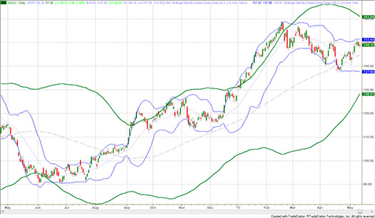
Figure – 3: One-Year Daily Chart of GS with standard Bollinger Bands
Blue: Daily Bollinger Bands, Green: Weekly Bollinger Bands
(click here to see a high-resolution version of this chart)
Figure 3 is the same price chart as Figure 2 with the addition of weekly Bollinger Bands plotted in green. The weekly Bollinger bands clearly show how they influence and usually contain the lower time frame daily Bollinger bands. Notice that in early 2013, the high momentum trend put price bars outside the weekly band and kept them there for two months while the daily Bollinger Bands still contained prices. The weekly bands put the move in the proper context of momentum which otherwise might have been less distinguishable.
Modified Bollinger Bands
Any volatility measure based on historic data including Bollinger Bands, expand quickly after a volatility increase but contract more slowly as volatility declines. The Achilles heel of Bollinger Bands is the time it takes for them to contract after volatility drops off, which makes trading some instruments using Bollinger Bands alone difficult or less profitable. You would need other techniques in a conventional Bollinger Band system to make it workable.
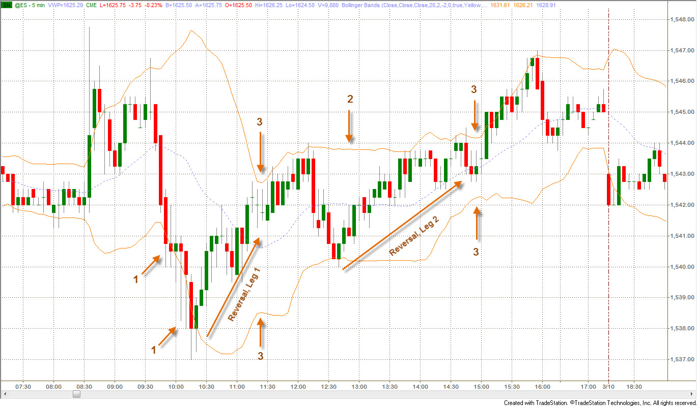
The chart below illustrates this problem:
- Initial Move: Bands quickly expand as volatility expands in section 1.
- Reversal Legs: The Bollinger Bands do not contract quickly enough to allow the trader to capture much of reversal leg 1. Traders must use another indicator to find the first reversal up from the bear move or rely on skillful reading of the price action.
- Squeeze: A minor Bollinger Band squeeze pattern occurs at about 11:20 (point 3 on the left), but by then, half of the bull reversal move has happened already. If you consider the more significant squeeze at about 15:00 (point 3 on the right), two-thirds of the move was missed.

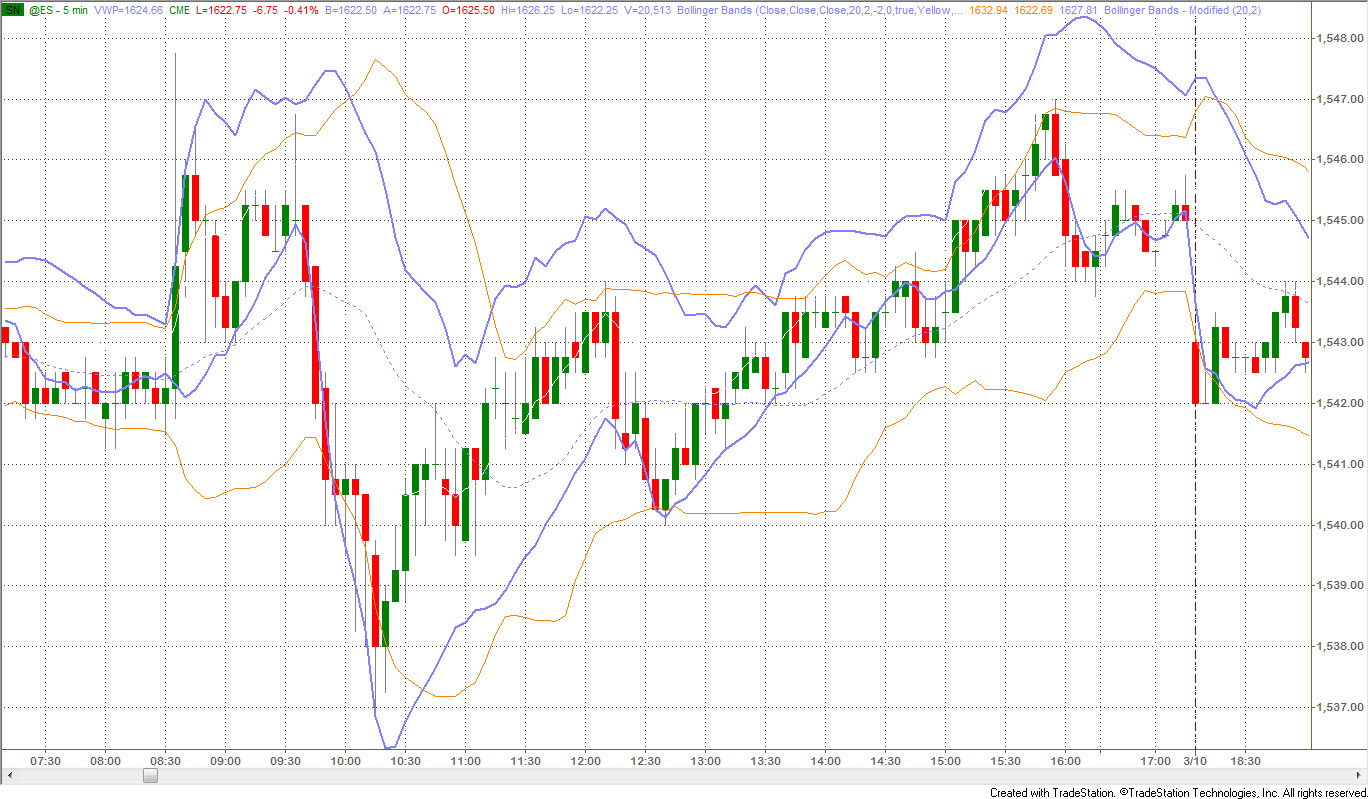
Figure – 4: Standard Bollinger Bands on a 5-Min Intraday Chart of ES (March 8, 2013): notice the slow contraction of these bands incurs delay in trader’s decision making.
(click here to see a high-resolution version of this chart)
It is possible to correct this problem. Dennis McNicholl wrote about a new method for calculating Bollinger Bands in an article: “Better Bollinger Bands” (Futures Magazine, October 1998). McNicholl recommends improving Bollinger Bands by modifying:
- the center line formula and
- different equations for calculating the bands.
The bands follow price more closely and respond faster to changes in volatility with these modifications.*
The chart below compares the conventional Bollinger bands in orange to the McNichol modified bands in blue. You can see how the bands contract more quickly after volatility expansions though there still is a lag.
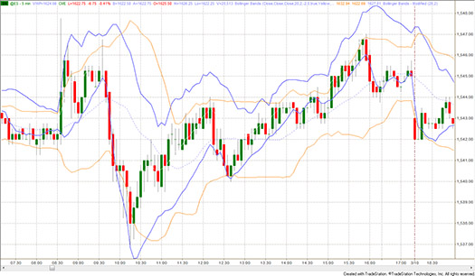
Figure – 5: 5-Min Intraday Chart of ES (March 8, 2013) with both Modified and standard Bollinger Bands:
notice the fast response of modified bands compared to standard ones.
(click here to see a high-resolution version of this chart)
Better Bands Yet
We built upon the concept of trends from part 1 and discussed some of the more popular trading bands and core techniques for trading them in this article. The most complex and advanced band construction technique is based on statistics rather than factors of price only. The third article in this series will be dedicated to this subject.
*The following short code for TradeStation plots a modified Bollinger Band based on McNicholl’s formulas:
{ Modified Bollinger Bands: from "Better Bollinger Bands" by Dennis McNicholl, "Futures," October 1998}
inputs: period(20), factor(2.0);
vars: alpha(0), m1(0), ut(0), dt(0), m2(0), ut2(0), dt2(0), but(0), blt(0);
{ smoothing constant }
alpha = 2/(period + 1);
mt = alpha*close + (1 - alpha)*m1;
ut = alpha*m1 + (1 - alpha)*ut;
dt = ((2 - alpha)*m1 - ut)/(1 - alpha);
mt2 = alpha*absvalue(close - dt) + (1 - alpha)*m2;
ut2 = alpha*m2 + (1 - alpha)*ut2;
dt2 = ((2 - alpha)*m2 - ut2)/(1 - alpha);
but = dt + factor*dt2;
blt = dt - factor*dt2;
{ plot bands }
plot1(dt,"center");
plot2(but,"upper");
plot3(blt,"lower"); |
About the Author: Ali is an IT architect based in Toronto, Canada. He started trading options in 2006. Despite early success, he realized he needed both a deeper understanding of self and of trading to ensure continued success. Reading Dr. Tharp’s books brought him to Cary to take part in various IITM courses. Ali has spent the past five years studying and perfecting his trading. He is planning to move to full time trading after completing his current technology consulting project.
Trading Education
The Frog day-trading system has multiple intraday opportunities every day the market is open. Positions are closed by the end of the day, so there’s no overnight risk or worrying about positions while you lay in bed at night. The Frog system is part of the Day-Trading Workshop in August.
July 13-14 |
Core Trading Systems
Longer Term Trading Systems from Ken Long
Even if you intend to trade shorter term, this workshop acts as a rock-solid foundation to trade swing systems later on.
|
| August 10-11 |
Oneness Awakening Weekend
with Van Tharp
Just Announced! |
August 16-18 |
Day Trading Systems
with Ken Long
Learn Ken's Frog and RLCO systems
|
August 19-21 |
Live Day Trading
with Ken Long
Day Trading Systems is a prerequisite to this course.
|
October 3-14 |
Peak Performance 101, 202 and 203
Register for Peak 101 and get on the waiting list for 202 and 203 now.
|
| Berlin, Germany Workshops |
September 6-8 |
How to Develop a Winning Trading System
with Van Tharp and RJ Hixson
|
September 10-12 |
Blueprint for Trading Success
with Van Tharp and RJ Hixson
|
September 14-16 |
Forex Trading
with Gabriel Grammatidis
|
Register for all 3 and save $800!
|
To see the full schedule, including dates, prices, combo discounts and location, click here.
Trading Tip
A Deeper Look at Unemployment Numbers: Part 2
by D. R. Barton, Jr.
View On-line
By the time you read this article, the Federal Open Market Committee (FOMC) will have completed its meeting, made its announcement, and Ben Bernanke will have tap-danced through another “post-Fed” press conference. Since I submitted this article well before all of those shenanigans occured, there was no need for me to have speculated on what the Bernanke said — you’ll already know by the time you read this.
If you will, however, allow me one or two predictions. We can be fully sure that pundits and talking heads will dissect every syllable and nuance, and the market will jump up and down for a while during and after said dissection. Most likely, the Fed will hold the course and say that any tapering (or other euphemism for reducing the morphine-like monthly monetary injection) will not be happening in the near-term. They will also have to address the economic picture in general and the employment picture in particular. We looked at one aspect of the unemployment situation last week and this week, we’ll continue on that subject a bit more.
Wow — There Are a Lot of Unemployed Folks Out There…
Last week, we discussed how “maximizing employment” is part of the Fed’s dual mandate from congress. And, no doubt, the Fed has just talked about an improving employment picture, since the Bureau of Labor Statistics’ (BLS) chart looks something like this:
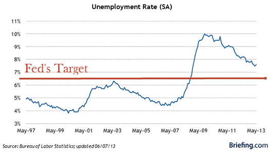
Before we get into analyzing this chart, here’s an interesting point — you’ll see that the Fed's targeted threshold level of 6.5%, the driver for the current monetary policy, is above the highest unemployment level hit during the decade before the real estate bubble burst.
The “SA” in parentheses in the title stands for “seasonally adjusted”. In theory, adjusting the unemployment rate for seasonal factors makes some sense. For example, one would expect lower unemployment around the Christmas shopping season. In practice, SA has become just another lever for policy wonks to pull and pundits to discredit.
On the other hand, are there problems with looking at completely unfiltered data? Sure. For example, I grew up in the classic nuclear family: my dad had a good, professional position at the local manufacturing plant and my mom stayed at home and raised three kids in exemplary fashion. Was she really “unemployed”? She worked harder than anyone I knew between running the household and volunteering for ministry and for other various causes. But by any economic measure she would be considered unemployed. She did not desire “normal” employment in the form of a wage earning job, so she really wasn’t a “participant” in the labor market.
So while various filters may be required, the way that some are thrown on the data to show a rosier employment picture is downright insane. The worst example of a misused filter comes from the now infamous Labor Force Participation Rate. It tries to address issues like whether my mom should have been counted, but it does it in a manner that doesn’t keep up with current trends (and it’s actually so interesting that we might just tackle it in depth next week…).
For those of you who read last week’s article, I’m sure you’re wondering how the U.S. numbers compare to the less-filtered numbers we presented for the European Union. To be fair, all of the European countries’ published unemployment numbers similarly have layers upon layers of filters. But I think the employment rate of all employable folks is an interesting way to look at the numbers so let’s jump back to a country comparison as provided by the very nice data library at the Organization for Economic Co-operation and Development (the OECD).
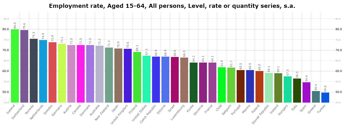
Here is the 4th quarter of 2012 chart that includes the U.S., the EU countries we looked at last week and a few other notables (Japan, Australia, Canada, etc.):

(click here to see a larger version of this chart)
We can see a similar pattern here to last week’s chart with higher employment generally in the northern and western European countries and lower figures for the southern and eastern states in Europe. You’ll also notice that the BLS unemployment figure at about 7½% does not translate into a 92½% employment rate by measures the OECD used. By the OECD measurement, the U.S. is about middle of the pack in employment compared to the other countries in the study.
OECD numbers aside, the Fed remains committed to a decision-making process tied to a 6.5% BLS unemployment figure. As long as this number continues to drive their strategy, it will continue to be of primary importance to the equities markets.
Since the BLS employment figure is so significant right now, it’s probably worth peeling this data onion back one or two more layers next week.
As always, your comments and feedback are welcome! Please send your thoughts to drbarton “at” vantharp.com
Great Trading,
D. R.
About the Author: A passion for the systematic approach to the markets and lifelong love of teaching and learning have propelled D.R. Barton, Jr. to the top of the investment and trading arena. He is a regularly featured guest on both Report on Business TV, and WTOP News Radio in Washington, D.C., and has been a guest on Bloomberg Radio. His articles have appeared on SmartMoney.com and Financial Advisor magazine. You may contact D.R. at "drbarton" at "vantharp.com".
Disclaimer
 Gold Report Gold Report
Gold Analysis and Strategy: June 17, 2013
by Florian Grummes
From time to time we'll share Florian's report with you. Click here to see the June report.
About the Author: Florian Grummes (born 1975 in Munich) has been studying and trading the gold market since 2003. In addition to his trading business, he is a very creative and successful composer, songwriter and music producer.
Ask Van...
Everything we do here at the Van Tharp Institute is focused on helping you improve as a trader and investor. Consequently, we love to get your feedback, both positive and negative!
Click here to take our quick, 6-question survey.
Also, send comments or ask Van a question by clicking here.
Back to Top
Contact Us
Email us at [email protected]
The Van Tharp Institute does not support spamming in any way, shape or form. This is a subscription based newsletter.
To change your e-mail Address, e-mail us at [email protected].
To stop your subscription, click on the "unsubscribe" link at the bottom left-hand corner of this email.
How are we doing? Give us your feedback! Click here to take our quick survey.
800-385-4486 * 919-466-0043 * Fax 919-466-0408
SQN® and the System Quality Number® are registered trademarks of the Van Tharp Institute
Be sure to check us out on Facebook and Twitter!
 
Back to Top |